I revamped my photon mapping system a few weeks ago. The results are now radiometrically correct, converging to the same image as path tracing. I currently support Lambertian diffuse reflection (for indirect diffuse) as well as ideal specular reflection and refraction (for caustics). I took some inspiration from progressive photon mapping, storing all photons (diffuse and caustic) in a single photon map, visualizing the photon map directly (instead of doing final gathering), and doing multiple passes and progressively improving the image. Currently, I'm using a fixed search radius for photon lookups (and my own templatized k-d tree), and just starting with a very small radius so that the results are visually indistinguishable from path tracing; I could easily modify the system to use an increasingly smaller search radius. Because I'm doing multiple passes, memory isn't an issue—I can trace any number of photons in each pass, which affects the rate of convergence, but not the final result.
My old photon system had some significant limitations and flaws. When I started working on my ray tracer over two years ago, I thought photon mapping would be the best way to achieve realistic lighting, but I knew very little about rendering and radiometry at the time, so while I made good progress on it, I was not able to implement everything correctly or efficiently, and I eventually got stuck. Now I have a better understanding of that stuff, so I revisited photon mapping, partially for the fun and challenge, and partially to produce pictures that I couldn't produce before—pictures of situations that are difficult for path tracing to handle, especially caustics from small, bright lights.
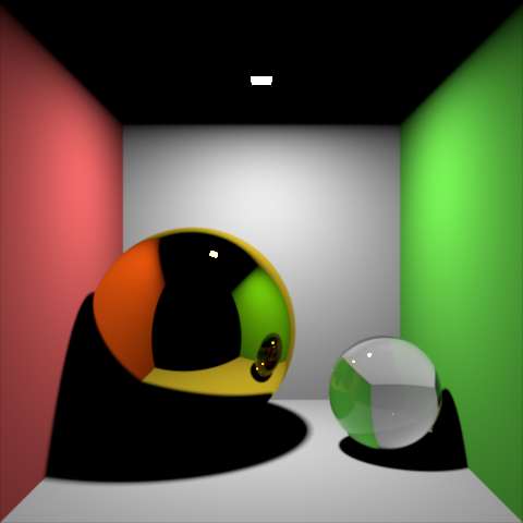
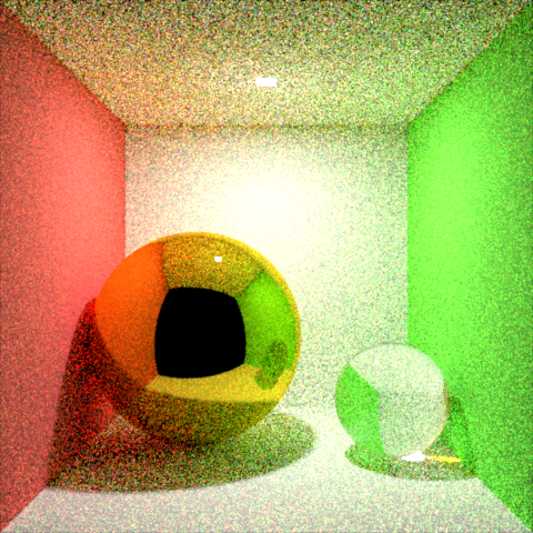
I plan to make my photon mapping system more powerful in the future, and to render some pretty images containing fancy caustics. The scene I rendered below is not the most attractive, but it's good for illustrative purposes.
 |
| Photon mapping used for indirect diffuse and caustics. |
 |
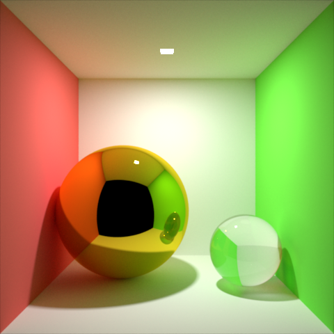
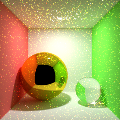
| Path tracing reference. Looks identical to the photon mapping version above, except it's still a little noisier than the photon mapping version. I let this render for much longer than the photon mapping version. The caustics took forever to smooth out. |
 |
| Path tracing with photon-mapped caustics. |
 |
| Direct lighting only (plus specular reflection and refraction of camera rays). In the top image above, all of the rest of the light comes from the photon map. |
 |
| Path tracing with no caustics. Compare to the full versions above to see how much contribution caustics have on this image. Also notice the lack of noise, even though this was rendered in much less time than the full path tracing image above. |
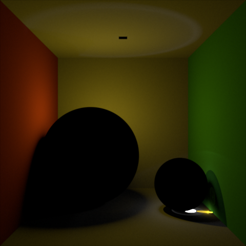 |
| Caustics only (created using photon mapping). |
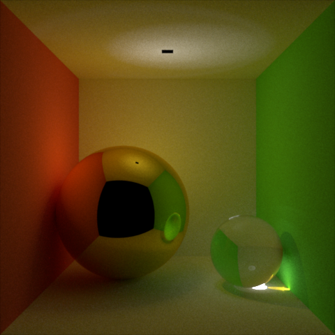 |
| Caustics, plus diffuse and specular reflection and refraction. This is what the scene looks scene looks like if lit only by the caustics in the image above. Notice, on the ceiling, the caustic of a caustic; the hot spot under the glass ball is projected back through the ball and onto the ceiling. |
 |
| What the top photon mapping image looked like after the first pass. |
 |
| What the path tracing reference looked like after the first pass (which took quite a bit longer than one pass of the photon mapping version). The fireflies are the caustics. |
 |
| Subtle artifacts (isolated here) from a pseudo-random number generator issue. Months ago I changed my PRNG to Mersenne Twister, but I switched it back to rand() when I put the program on my Mac laptop to work on it on it over the summer, because the Mersenne Twister stuff didn't port without effort. It took me a while to figure out what was causing these artifacts. |
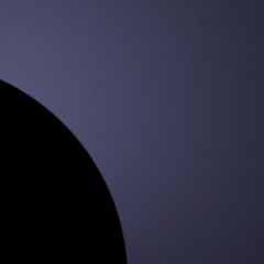 |
| Problem fixed by switching Mac version to use Mersenne Twister. |
nice work!
ReplyDeleteHey, thanks Xing!
DeleteVery nice! The bit with the artifacts from not using the Mersenne Twister is very curious, are those artifacts that arise from the nature of rand() itself, or just from not enough convergence?
ReplyDeleteThanks Karl!
DeleteIt actually converges to those artifacts—they are hardly visible at first, and then they crystallize with more samples. From what I could tell from a few tests, there was a correlation between the location on the light that a photon was emitted from, and the direction that the photon was emitted in. In the test above, I color-coded the photons based on where they were emitted from the light, and you can see that the brighter parts of ripples are more purple, while the darker parts are more blue (confirmed in Photoshop by extracting the hue). Seems like the problem was only evident in the caustics because the rays stay coherent when they bounce off of the ideal specular sphere—otherwise there's nothing special about the caustics. I was able to see a similar crisscrossed ripple pattern in these caustics with backwards path tracing when I injected some rand() influence on Windows (where my compiler has a RAND_MAX of only 32767). In general, rand implementations don't use the highest quality PRNGs (sounds like rand_s on Windows might be better though).
Search for Linear Congruential Generators in Wikipedia to read about the problems with the low quality PSRNs you have found
ReplyDeleteVery interesting! Thanks for the pointer, RC.
DeleteHi there. Nice work :). How do you address the photon mapping problem of including photons from other surfaces (edges, corners)? Are you doing the direct illumination using standard techniques i. e. like in PT?
ReplyDeleteThanks for the comment Michal. To address the problem of including photons from other surfaces, I do two main things:
Delete1. Weight samples based on the similarity of the surface normal and the photon normal. (Based on your blog, it sounds like you've done something similar in your own renderer.)
2. Make the search radius small enough that the problem isn't noticeable.
Yes, I'm doing direct illumination using standard techniques.
Nicely done! I learnt a lot from reading your process! Did you use sphere or disc or cube for photon gathering? Are there any filter kernels applied? (If not, is the smooth result comes from multiple passes?)
ReplyDeleteThank you for the comment!
DeleteTo estimate the irradiance at a point on a surface, I first gathered all of the photons within a sphere of a small fixed radius. Then I made the assumption that all of the gathered photons lay on a flat disc. This allowed me to compute the irradiance by summing the power of all of the gathered photons and dividing by the surface area of the disc. The radius of the disc was assumed to be the same as the search radius, and the normal of the disc was assumed to be the same as that of the surface at the ray intersection point. This is a pretty good approximation when the radius is really small relative to the variation of the surface normal.
I didn't apply any filter kernels. That's correct: the smooth result comes from multiple passes, each with lots of photons.
Thanks for your reply!!
DeleteI'm more curious about your multiple pass estimation~ Did you scattered multiple times, build several kdtrees to store photons (I assume), and do multiple passes of irradiance estimation with same parameters (like how many photons per intersection, maximum sampling radius)? Or did you use the same kdtree, and do multiple irradiance estimation with sampling in different parameters?
I tried so hard to get the super nice looking and accurate caustics in your caustic only image! But my method (Jensen's, in which I try to gather a certain number of photons and estimate irradiance with the radius of the farthest photon of sample set) lost details of caustics. The caustic under the transmissive sphere is more like some very bright spots.
Sorry if I made some confusion... I combined my blogspot account 棋坪的顾渚紫笋 with my google account :P
DeleteHey Xiao,
DeleteIn each pass, I scattered new photons and built a new k-d tree. Each pass used the same parameters (the same maximum sampling radius) but different photons.
I did not decrease the search radius in each pass as in progressive photon mapping. That would have been a consistent algorithm, but it also would have introduced additional bias at the beginning of the render that would have had to have been overcome with more passes.
Instead, I started with a very small search radius. That was the key to the very sharp, detailed caustics. Because of the small radius, the image started out with a lot of high frequency noise, but eventually converged to something smooth and sharp.
I estimated the irradiance using all of the photons inside the fixed search radius, not just the farthest photon. This should make the image converge faster than using only one, since all of the photons typically have different powers. Also, gathering all of the photons inside a fixed search radius instead of gathering a certain number of photons ensured that the distance to the gathered photons was small, which ensured that the caustics would be sharp and not blurred out, even in areas of low photon density.
Thank you Peter! You have a very interesting approach and it sounds reasonable! I implemented your method, with 500,000 photons both for global illumination and caustics each pass, and in total I tried 10 passes and 50 passes. For each pixel, I summed up the colors from all passes and divide it by total pass amount.
DeleteMy final result still has a lot of noises, and the smoothing is prominent for the first 5 passes, after that, the noises seems staying there for ever. Did you have such a problem in your work? Also I'm not sure if my way of averaging the color from every pass is correct for convergence?