Bidirectional Path Tracing and Metropolis Light Transport

During my last semester at Penn I implemented bidirectional path tracing and Metropolis light transport (MLT). My bidirectional path tracing implementation is based on Eric Veach's PhD thesis and includes all of the possible sampling techniques (including the more difficult cases such as when the light subpath intersects the sensor), complete multiple importance sampling (MIS), and a variety of other optimizations. I implemented Kelemen-style MLT on top of bidirectional path tracing. I also implemented some new BSDFs, including the Disney "principled" BSDF, and I improved my implementation of the microfacet BSDF for transmission through rough surfaces. I implemented all of these things in a separate, streamlined version of Photorealizer. Now I have two separate renderers, which I would like to merge together at some point.

I documented this project in a separate blog: http://bptmlt.blogspot.com/

An image I rendered using bidirectional path tracing in my newest renderer. See my project blog for details.

An image I rendered using bidirectional path tracing in my newest renderer. See my project blog for details.

Eliminating Dark Edges When Using a BSSRDF

The edges and corners of an object shaded using a BSSRDF tend to be dark compared to the rest of the object. I recently came up with a way to fix these dark edges and corners.

First I investigated exactly what causes dark edges. They are not typically caused by an inadequate number of irradiance samples. And they are not typically caused by the lack of single scattering—single scattering can brighten edges a little bit (since light there is more likely to enter and exit before being absorbed) but not enough to counteract the darkening effect. I discovered that, in many cases, the actual problem is not that the edges are too dark, but that the other regions are too bright. The reason that some regions are too bright or too dark is that too much or too little incident light is being considered when evaluating the diffusion approximation. My new method fixes bright and dark regions.

Using a BSSRDF involves integrating the incident radiance not only over the hemisphere above a point (as with a BRDF), but also over the surface around the point. The diffusion approximation BSSRDF that I am using is designed to work with flat, semi-infinite slabs of material. The contribution of any infinitesimal surface patch is a function of the area of that surface patch and the distance to the point being shaded (among other things). The result ends up too bright when the surface around the point being shaded is wrinkly or contains faces from other sides of the object. In those cases the surface area within any given distance is larger than it would be if the surface were flat, and the diffusion approximation gives a higher result. In addition to looking bad, this can cause violations of energy conservation by adding energy to the system. Furthermore, the result ends up too dark in thin areas where there is less surface in the vicinity of the point being shaded than there would be if the surface were flat.

To fix this, I normalize the result so that it looks the way it would look if the surface were flat. Before rendering begins I numerically integrate the BSSRDF over the a hypothetical infinite flat surface to find the total diffuse reflectance (which I use in place of the multiple scattering component during the irradiance computation pre-pass). Then during rendering, when I evaluate the diffusion approximation for real, I keep track of two things: the value it actually yields, and the value it would yield if the irradiance were 1 everywhere on the surface (which, in the case of a flat surface, is the same as the total diffuse reflectance). Then I divide the regular result by the ratio of the irradiance=1 result and the total diffuse reflectance (the flat surface irradiance=1 result). This fixes the geometry-dependent brightness variations, and gives the BSSRDF the appearance of simply blurring in space the results of a diffuse BRDF that uses the total diffuse reflectance as its albedo.

It's possible that others have done similar things in the past, but I haven't heard of it myself.

(Sorry if some of that description is unclear. I should make another pass over this post to improve it, but I wanted to get it posted sooner rather than later.)

Below are some renders that illustrate the results: a BRDF render, followed by three normalized BSSRDF renders, followed by an unnormalized (regular) BSSRDF render, followed by cropped versions of the last normalized render and corresponding unnormalized render. Click an image to bring up the lightbox, then switch between images to compare them back-to-back. The differences are most evident when switching between images in this way.

Completely opaque marble. BRDF used instead of BSSRDF.

 Translucent marble created using a BSSRDF and my new normalization scheme. 

Same as the image above except with scattering and absorption coefficients cut in half.

Same as the image above except with scattering and absorption coefficients cut in four.

Same as the image above except without my new normalization scheme. Notice the differences in the wingtips, the torch, the fingers, the torso, and the folds in the lower part of the dress.

Close-up of the most translucent statue with normalization.

Close-up of the most translucent statue without normalization. Without normalization, the torch and wing tip are too dark, while the body and lower wing are too bright.

Another close-up of the most translucent statue with normalization.

Close-up of the most translucent statue without normalization. Without normalization the fingertips are too dark and other areas are too bright.

Bonus Renders

Here are some more renders that I've created with my updated subsurface scattering and dispersion systems.

First, a smoother, more translucent bunny. Compared to the bunnies from two posts ago, this bunny has lower scattering and absorption coefficients, and it exhibits forward scattering instead of isotropic scattering.

Path-traced subsurface scattering.

Next, a diamond ring with dispersion. The dispersion in these particular diamonds is relatively subtle because the lighting is very flat, and because the lighting and objects are all shades of gray. All of the color comes from dispersion.

Diamonds with dispersion. Ring designed by Alice Herald, © 1791 Diamonds.

I also rendered updated versions of the translucent blue Lucy images that I rendered last year. You can see the original images here.

Subsurface scattering accomplished using Monte Carlo path tracing.

A diffuse, opaque approximation of the image above.

BSSRDF-based multiple scattering + single scattering.

Before creating the approximate version (the last image), I made some speed and memory optimizations to my BSSRDF-based multiple scattering system. In particular, I now cache all of the values that are the same every time the BSSRDF is evaluated. 

Better Dispersion

Photorealizer now has high quality, physically accurate, spectral dispersion.

I improved the dispersion system in Photorealizer using some ideas that I wrote about in two old posts and a comment (here, here, and here). Instead of just tracing rays for RGB primaries, I now trace rays across the entire visible spectrum. Most parts of Photorealizer still use RGB color, but when a dispersive material is encountered, I choose a single wavelength from the visible spectrum, determine the index of refraction using the Sellmeier equation, and then continue path tracing with that wavelength. Then I convert the results to sRGB primaries using the spectral responsivity curves of the camera's RGB sensor. I derived these spectral responsivity curves from the new physiologically relevant CIE XYZ color matching functions (which I wrote about in this post on my sky renderer blog), and normalized them such that pure white light (containing equal amounts of all the wavelengths of the visible spectrum) is transformed into pure white in the sRGB color space (1,1,1) (i.e., I made each curve integrate to one). The spectral responsivity curves can take on negative values, and I don't clip negative color components until a bitmap image is output, which allows colors outside the sRGB gamut to be represented using the sRGB primaries. While these negative colors can't be displayed on a typical display, they are still useful and necessary for accurate color math. For example, adding a positive color to a negative one can result in a positive color in the displayable range, but if the negative color had been clipped to zero the result of the addition would be different and wrong.

I rendered new images of diamonds using my improved dispersion system. These images are 1600x900. You can click on an image to enlarge it, or you can open an image in a new tab or download it to ensure that you are viewing it at full size.

Diamonds with dispersion. The scene is completely grayscale; all of the colors in the image come from dispersion. Click to view at full size and see all of the colorful details.

Diamonds without dispersion.

Diamonds with dispersion but without transmission.

Highly saturated version of the image above, to clearly show that dispersion affects reflection, not just refraction (higher frequency (i.e., bluer) → higher index of refraction → higher reflection coefficient).

An old dispersion render (from this post) in which I traced only 3 specific wavelengths: 1 for red, 1 for green, and 1 for blue. (There are some other differences between this and the new render as well.)

Subsurface Scattering Improvements

I recently made some significant improvements and additions to Photorealizer's subsurface scattering (SSS) capabilities. In particular, I implemented the following:

• separate scattering coefficients for R, G, and B channels (for both path-traced and diffusion-based SSS)
• the Better Dipole model (for more accurate diffusion-based SSS)
• basic single scattering (for use with diffusion-based SSS)
• several bug fixes (for diffusion-based SSS)

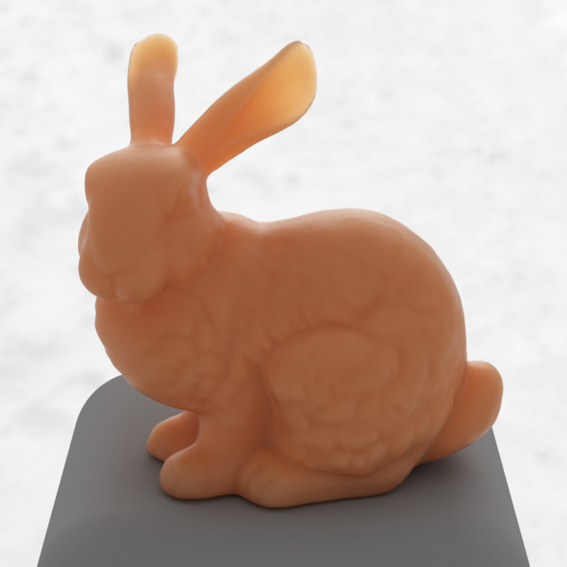
Below are some new Photorealizer renders showing off the new features. Click the images to view them at full size and do back-to-back comparisons. The strong transfer curve I've applied might slightly exaggerate the differences between the path tracing and diffusion versions.

Path tracing.

Diffusion-based multiple scattering plus single scattering.

Diffusion-based multiple scattering only.

Diffuse BRDF approximation to multiple scattering.

Diffuse BRDF approximation plus single scattering.

Single scattering only.

No transmission at all.

Miscellaneous Details

Below are some miscellaneous details about my SSS systems.

My Monte Carlo path tracing SSS system is unbiased and physically-based. I use the Henyey–Greenstein phase function for anisotropic scattering. I currently support only homogeneous media, although I could use unbiased distance sampling (which I implemented in my sky renderer) for heterogenous media. In the updated system, when the R, G, and B scattering coefficients differ from one another I trace separate rays for the separate channels.

As I've described in previous posts, my diffusion-based SSS system uses a precomputed, hierarchical point cloud of irradiance samples. The system works with multiple objects and even instancing—I create a separate point cloud for each object that is marked for diffusion-based multiple scattering.

To compute the albedo for the diffuse BRDF approximation for the Better Dipole model, I used numerical quadrature, rather than trying to do analytical integration. This only needs to be done once for each material, so it has no noticeable impact render times.

Several of the resources that I've been using for diffusion-based SSS have lots of ambiguities and some errors. By cross-referencing various sources and closely examining the derivations of the models, I was able to identify several things that needed to be fixed in my implementation. I did some relatively extensive testing, and I believe that all of the major pieces of my implementation are now correct. As a result, my renders are now much more physically-accurate.

My diffusion and path tracing renders still don't match perfectly due to the limitations and inaccuracies of the dipole diffusion approximation. The dipole diffusion approximation assumes that the object is a semi-infinite, homogeneous slab, and does not handle thin or curvy geometry well. In the model, light is forced to a depth of one mean free path before scattering, which is especially inaccurate near the source, blurring away fine details and causing low albedo colors to be absorbed too much. Some light goes all the way through the object, and this is not handled properly. Further inaccuracies are inevitable due to other assumptions that the model makes and approximations made in the derivation. Path tracing is still the best option when you want the most accurate results—it captures all of the subtleties automatically, and the resulting images have noticeably more depth.

Test Renders

Below are some test renders. The scene is a top-down view of a large slab of material. The material scatters and absorbs all wavelengths equally. There is a magenta environment map surrounding the scene (which is why the material looks magenta). In the upper right, there is a green spherical emitter. The black line is a thin wall that prevents light from the sphere from passing to the other side except by way of SSS. In other words, all of the green to the right of the wall is a result of subsurface scattering.

First 4 images:

Relative IOR: 1.62

Phase function: isotropic

Single-scattering albedo: 0.999

Path tracing.

Diffusion-based multiple scattering plus single scattering.

Diffusion-based multiple scattering only.

Diffuse BRDF approximation to multiple scattering.

Next 4 images:

Relative IOR: 1

Phase function: isotropic

Single-scattering albedo: 0.999

Path tracing.

Diffusion-based multiple scattering plus single scattering.

Diffusion-based multiple scattering only.

Diffuse BRDF approximation to multiple scattering.

Final 4 images:

Relative IOR: 1

Phase function: isotropic

Single-scattering albedo: 0.667

Path tracing.

Diffusion-based multiple scattering plus single scattering.

Diffusion-based multiple scattering only.

Diffuse BRDF approximation to multiple scattering.

Instancing Render

Lots of airplanes, rendered in Photorealizer. Click to view big (originally rendered at 1920x1080, but Blogger has scaled it down to 1600x900).

I rendered the image above using my instancing and transformations system. There are multiple copies of the same airplane model. I arranged the planes procedurally, giving them translations and rotations and ensuring that they don't overlap.

There are 1272 planes in the scene. Without triangulation, that would have been a total of 100 million polygons. But I had Photorealizer triangulate the model which resulted in a total of 194 million triangles. With or without triangulation, the total number of vertices was 121 million—polygons in a mesh share vertices in Photorealizer.

The scene has a BVH that contains the planes, and the plane has it's own BVH that contains its geometry.

This is one of the first images that I've rendered using my improved transfer curve.

The image is a revised version of an image that I rendered in 2011, which you can see below. I probably prefer the lighting of the old version, the way it's lit by the sun, but I lit the new version differently so I wouldn't have to deal with caustics.

Old version.

Gold Bunny Lit by Sun and Sky

Close-up of photon contribution. Click to view large. (I originally rendered this image at 1618x1000, although Blogger has scaled it down to 1600x989, so there might have been a slight loss of quality.)

I rendered an image of a gold bunny lit by a sun and sky (the render from this post) that I rendered in my sky renderer. This was possible through the use of an HDR environment map, HDR environment map importance sampling, and HDR environment map photon emission. The top image below is the complete image—it contains all of the paths that light can take from the light source to the camera. The next image contains only direct illumination, as well as specular reflection of camera rays. The image after that shows only the photon contribution. Finally, the image above is a bigger, brighter, higher quality view of the photon contribution; a total of over one billion photons were stored in the photon map (not all at once) when creating that image.

All possible types of light paths.

Direct illumination, as well as specular reflection of camera rays.

Photon contribution.

Snow Globe Render

This year, I designed and created the cover image for the Penn Computer Graphics holiday card. I rendered the image in my renderer, Photorealizer:

The render features, among other things, global illumination accomplished with Monte Carlo path tracing, path-traced subsurface scattering, a 3D procedural wood texture, reflection from and transmission through rough surfaces, correct behavior at the glass–water (and other) interfaces, an HDR environment map, a spherical light, depth of field, anti-aliasing using a Gaussian reconstruction filter, and an S-shaped transfer curve.

Instead of using neutral white lights like I've often done in the past, I lit this scene with complimentary blue and yellow lights (glacier HDR environment map and small, bright spherical light respectively). This gives the image a more interesting and varied appearance, while keeping the light fairly neutral on the whole. When I started working on the lighting, I started with just the environment map and the image appeared far too blue. Instead of zeroing out the saturation of the environment map or adjusting the white balance of the final image, I decided to add the yellow spherical light to balance it out (inspired by the stage lighting course I took this past semester).

I spent some time tweaking the look of the snowflakes—the shape, the material, and the distribution. I ended up settling on the disc shape, which is actually a squished sphere (not a polygonal object). All of the snowflakes are instances of that same squished sphere. For the material, I made the snowflake diffusely reflect half of the incident light, and diffusely transmit the other half (in other words, a constant BSDF of 1/(2π)). This gives a soft, bright, translucent appearance, while still being very efficient to render (compared to subsurface scattering).

I made some different versions of the image to show how certain features affect the look of the final image:

Half-size version, for comparing to the images below.

White light version.

Display-linear version.

Opaque perfectly diffuse version
(statue, snowflakes, and tablecloth).

For best results, the model needed to be very clean, exact, and physically accurate. I chose to model it using Houdini. I think Houdini is a very well-made piece of software. I really like its node paradigm, procedural nature, and clean user interface. I like having the ability to set parameters using precise numbers, or drive them with scripts, and having the ability to go back and modify parameters in any part of the network at any time.

In addition to using Houdini, I created the LOVE statue shape in Illustrator, and I procedurally added the snowflakes in Photorealizer.

Here are screenshots of the Houdini network and the resulting model:

Houdini network.

Houdini model.